The province of Ontario has a great Open Data Initiative. While their online portal is easy to use, I thought I’d practice my scraping skills and create my own organized dataset of available datasets. Extracting information from the webpage is straightforward using the rvest package.
library(rvest)
library(dplyr)
library(ggplot2)
library(ggthemes)
Ontario has done a nice thing by letting all available datasets load on a single page. The steps below extract title, description, date, source, and link information from the list using CSS selectors (easiest to find using SelectorGadget in Chrome):
open.data <- "https://www.ontario.ca/open-data?query=&lang=en&type=dataset&pages=52#load510"

title <- open.data %>%
  read_html() %>%
  html_nodes(css = '#search_results a') %>%
  html_text()

desc <- open.data %>%
  read_html() %>%
  html_nodes(css = '.search_dataset_description') %>%
  html_text()

date <- open.data %>%
  read_html() %>%
  html_nodes(css = '.search_dataset_description+ .search_dataset_result_left') %>%
  html_text()

source <- open.data %>%
  read_html() %>%
  html_nodes(css = '.search_dataset_result_right:nth-child(4)') %>%
  html_text()
Once we have all the information, combine and clean: isolate the year of publication and focus on the non-repetitive part of the source column:
open.data <- cbind(title, desc, source, date, link)

open.data$date <- sapply(strsplit(open.data$date, split = ': ', fixed = TRUE), function(x) (x[2]))
open.data$release.year <- sapply(strsplit(open.data$date, split = ' ', fixed = TRUE), function(x) (x[2]))
open.data$source <- sapply(strsplit(open.data$source, split = ': ', fixed = TRUE), function(x) (x[2]))

write.csv(open.data, "ON_opendata.csv")
First, a figure showing what parts of the Ontario Public Service are contributing to the database:
source.counts <- count(open.data, source)

ggplot(data = source.counts, aes(x = reorder(source, n), y = n, label = n)) +
  geom_text(size = 3) +
  labs(x = "", y = "") +
  coord_flip() +
  ggtitle("Sources of Ontario Data") +
  theme_few() +
  theme(axis.ticks = element_blank(), axis.text.x = element_blank())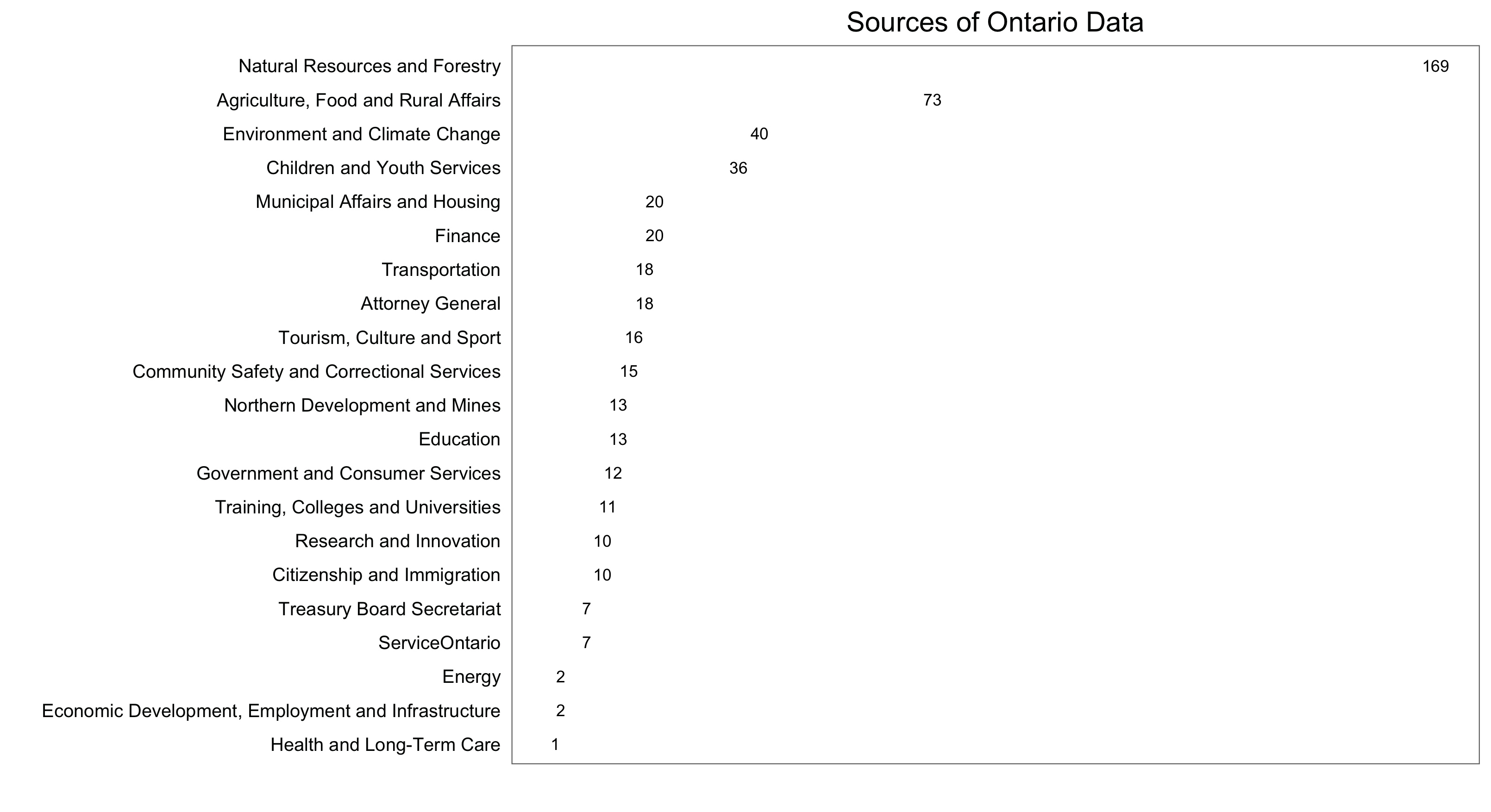
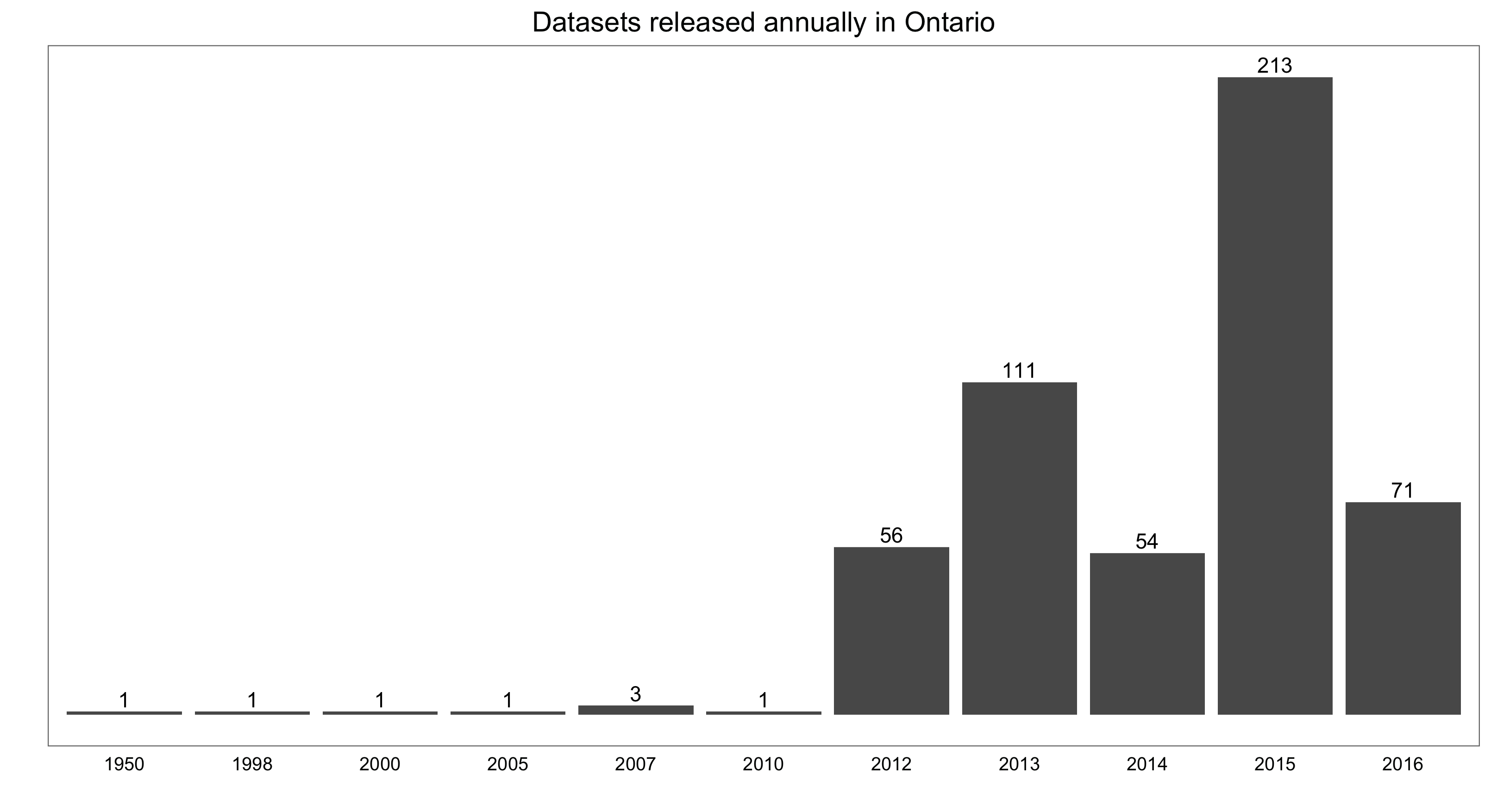
And a simple bar chart showing the number of datasets released by year:
year.counts <- count(open.data, release.year)

ggplot(data = year.counts, aes(x = release.year, y = n, label = n)) +
  geom_bar(stat = "identity") +
  geom_text(aes(label = n), vjust = -0.30) +
  labs(x = "", y = "") +
  ggtitle("Datasets released annually in Ontario") +
  theme_few() +
  theme(axis.text.y = element_blank(), axis.ticks = element_blank())