The province of Ontario has a great Open Data Initiative. While their online portal is very easy to use, I thought I’d practice my scraping skills and create my own organized dataset of available datasets. Extracting information from the webpage is pretty easy using the rvest package.
library(rvest)
library(dplyr)
library(ggplot2)
library(ggthemes)
Once packages are loaded, we specify the link we want to scrape from. Ontario has done a nice thing by letting all of the available datasets load on a single page; it took some trial and error, but I hit on a URL that gets them all listed together.
open.data <- "https://www.ontario.ca/open-data?query=&lang=en&type=dataset&pages=52#load510"
Once the URL is loaded we are away to the races. The easiest way to find css (or xpath) tags for the relevant information on the page is using a Chrome plugin called SelectorGadget. The steps below extract title, description, date, source, and link information from the list.
# Titles
title <- open.data %>%
  read_html() %>%
  html_nodes(css = '#search_results a') %>%
  html_text()
title <- data.frame(title, stringsAsFactors = F)

# description
desc <- open.data %>%
  read_html() %>%
  html_nodes(css = '.search_dataset_description') %>%
  html_text()
desc <- data.frame(desc, stringsAsFactors = F)

# date published
date <- open.data %>%
  read_html() %>%
  html_nodes(css = '.search_dataset_description+ .search_dataset_result_left') %>%
  html_text()
date <- data.frame(date, stringsAsFactors = F)

# source
source <- open.data %>%
  read_html() %>%
  html_nodes(css = '.search_dataset_result_right:nth-child(4)') %>%
  html_text()
source <- data.frame(source, stringsAsFactors = F)

# link
link <- open.data %>%
  read_html() %>%
  html_nodes(css = '#search_results a') %>%
  html_attr(name = "href")
link <- data.frame(link, stringsAsFactors = F)
base_url <- "https://www.ontario.ca"
link$link <- paste0(base_url, link$link)
Once we have all of the information we want to extract, it R makes it simple to combine and then clean them up a little bit. In this case cleaning means isolating the year of publication and focusing in on the non-repetitive information in the source column:
open.data <- cbind(title, desc, source, date, link)

open.data$date <- sapply(strsplit(open.data$date, split=': ', fixed=TRUE), function(x) (x[2]))
open.data$release.year <- sapply(strsplit(open.data$date, split=' ', fixed=TRUE), function(x) (x[2]))
open.data$source <- sapply(strsplit(open.data$source, split=': ', fixed=TRUE), function(x) (x[2]))

write.csv(open.data, "ON_opendata.csv")
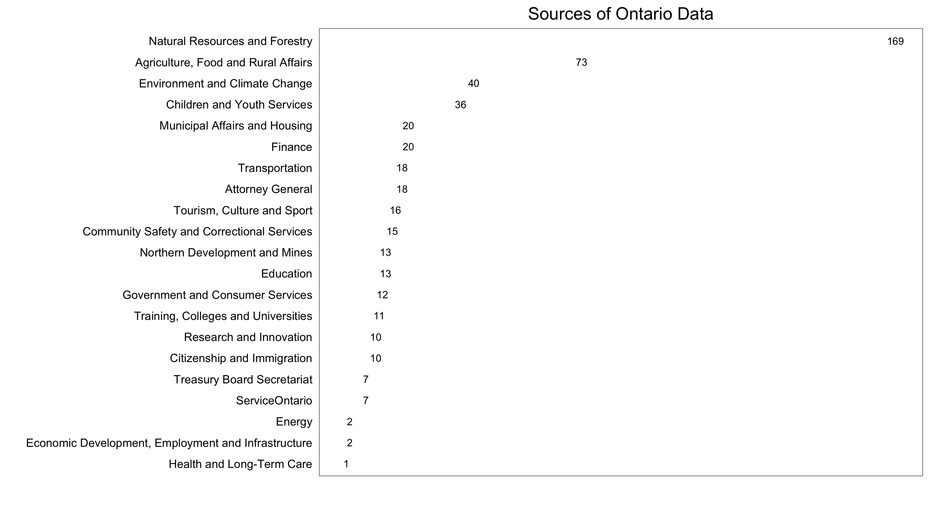
I won’t take it much further than that, but the last step above creates a .csv that you are welcome to explore yourself (available here). I’ll finish with a little metadata visualization: first, a figure that shows what parts of the Ontario Public Service are contributing to the database:
source.counts <- count(open.data, source)

ggplot(data = source.counts, aes(x = reorder(source, n), y = n, label = n)) +
  geom_text(size = 3) +
  labs(x = "", y = "") +
  coord_flip() +
  ggtitle("Sources of Ontario Data") +
  theme_few() +
  theme(strip.background = element_blank(),
        strip.text = element_blank(),
        axis.ticks = element_blank(),
        axis.text.x = element_blank())
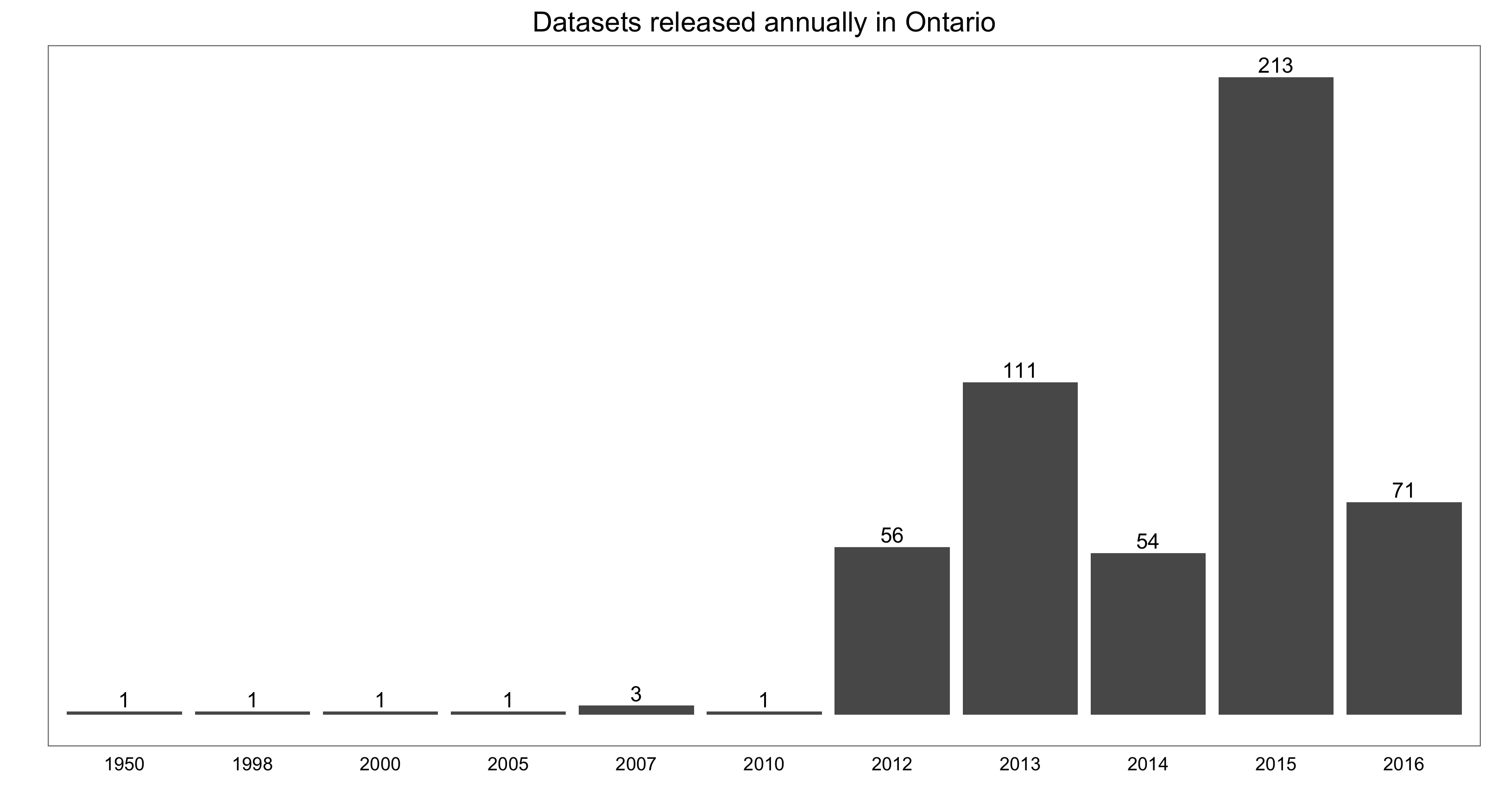
And second, a simple bar chart showing the number of datasets in the database by release year:
year.counts <- count(open.data, release.year)

ggplot(data = year.counts, aes (x = release.year, y = n, label = n)) +
  geom_bar(stat = "identity") +
  geom_text(aes(label = n), vjust=-0.30) +
  labs(x = "", y = "") +
  ggtitle("Datasets released annually in Ontario") +
  theme_few() +
  theme(strip.background = element_blank(),
        strip.text = element_blank(),
        axis.text.y = element_blank(),
        axis.ticks = element_blank())